Turtlegraphics with APL2

by Hendrik Rama and Martin Barghoorn

Transcribed from the printed issue; not yet reviewed. Read it in the PDF of the issue, page 104

Turtlegraphics are well known from the LOGO-System [1]. These graphics are also vector graphics not made by setting the absolute X-Y-coordinates but by relative increments of distances and angles. Perhaps with some new APL2-Idioms we have developed in a short time more than 1500 graphics from different classes.

Derivation of the Formulas¶

We start with the APL2-Syntax (polar form of complex numbers), five points, angle 90 degrees.

      5⍴1D90
0J1 0J1 0J1 0J1 0J1

Rotation by multiplication and accumulation

      +\×\ 5⍴1D90
0J1 ¯1J1 ¯1 0 0J1

Splitting the real and the imaginary part

      9 11∘.○+\×\ 5⍴1D90
0 ¯1 ¯1 0 0
1  1  0 0 1

Transpose for drawing X-Y-graphics

      ⍉9 11∘.○+\×\ 5⍴1D90
 0 1
¯1 1
¯1 0
 0 0
 0 1

We get a quadrat (square) Q1 and then we take TRANSLATE and MAGNIFY from GRAPHPAK to find the right position on the centre of the screen (100 × 74 pixels).

      DRAW 60 30 TRANSLATE 25 MAGNIFY Q1← ⍉9 11∘.○+\×\5⍴1D90

Without the complex-numbers-syntax we take Cosine and Sine.

      Q2← ⍉ +\2 1 ∘.○ +\5⍴ ○ 90÷180   ⍝ COS, SIN

An alternative method is

      Q3← ⍉ +\2 1 ∘.○○ +\5⍴ .5        ⍝ COS,SIN,ALTERNATIVE

Proof

      (Q1≡Q2) (Q2≡Q3) (Q1≡Q3)
1 1 1

Different shapes of polygons (different classes)¶

      +\×\ 4⍴1D120  ⍝ Triangle
      +\×\ 5⍴1D90   ⍝ Quadrat (square)
      +\×\ 6⍴1D72   ⍝ Pentagon
      +\×\ 7⍴1D60   ⍝ Hexagon
      +\×\ 9⍴1D45   ⍝ Octagon

Rosettes¶

The application of the replicate-function generates multiple sets of data.

      ⍉9 11∘.○+\×\ 5 9/1D90 1D¯45

To get closed figures we need replications and further manipulations.

FIG 1: ⍉+\2 1∘.○○+\∊12/⊂(7+⍳7)/7⍴2 ¯2÷3 4
FIG 2: ⍉+\2 1∘.○○+\∊17⍴⊂(3+⍳4)/4⍴2 ¯2÷8 4
FIG 3: ⍉+\2 1∘.○○+\∊8⍴⊂(5+⍳9)/9⍴3 ¯1÷6
FIG 4: ⍉+\2 1∘.○○+\∊8⍴⊂(5+⍳7)/7⍴3 ¯1÷6
FIG 5: ⍉+\2 1∘.○○+\∊7⍴⊂(5+⍳8)/8⍴3 ¯2.5÷6

Trees [2]¶

VIS: Visibility, first column of the matrix

FIG 6: AX←,⊃.7×∘.,/4⍴(⊂1 1D15 1D¯15 1D30 1D¯30)
       AXX←⍉9 11∘.○AX1←2.5D90×∊0,+\×\⊃AX
       VIS←~0=AX1 ⋄ ERASE ⋄ DRAW VIS,30+8×AXX

FIG 7: AX←,⊃∘.,/5⍴⊂.5×(.03+(1 2D90 2D¯90.01)(1 2D¯90.01 2D90))
       AXX←⍉9 11 ∘.○ AX1←2.5D.0010×∊0,+\×\⊃AX
       VIS←~0=AX1 ⋄ ERASE ⋄ DRAW VIS,30+8×AXX

FIG 8: AXX←⍉9 11 ∘.○1D90×∊0,+\×\⊃,/,/.8,[2.5](.8D55 1D36
1D¯65)[⍉1+(5⍴2)⊤¯1+⍳32]
       VIS←~(0=AXX[;1])∧(0=AXX[;2])
       ERASE ⋄ DRAW VIS,40 +10×AXX

FIG 9: AXX←⍉9 11 ∘.○1D90×∊0,+\×\⊃,/,/.8,[2.5](.8D52 (.7D¯33
1D14).9D5)[⍉1+(4⍴3)⊤¯1+⍳81]
       VIS←~(0=AXX[;1])∧(0=AXX[;2])
       ERASE ⋄ DRAW VIS,30+10×AXX

FIG 10: AXX←⍉9 11 ∘.○1D90×∊0,+\×\⊃,/,/.8,[2.5](.8D52 (.7D¯33
.5D14 ¯1.1D14).9D5)[⍉1+(4⍴3)⊤¯1+⍳81]
       VIS←~(0=AXX[;1])∧(0=AXX[;2])
       ERASE ⋄ DRAW VIS,30+10×AXX

Patchworks¶

FIG 11: ⍉+\2 1∘.○○+\∊11⍴⊂(6+⍳10)/2÷(10⍴1 2 1)×.6
FIG 12: ⍉+\2 1∘.○○+\∊11⍴⊂(6+⍳16)/2÷(16⍴1 2 1)×.6
FIG 13: ⍉+\2 1∘.○○+\∊11⍴⊂(2+⍳12)/2÷(12⍴1 2 1)×.6
FIG 14: ⍉+\2 1∘.○○+\∊11⍴⊂(0+⍳7)/2÷(7⍴1 2 1)×.6
FIG 15: ⍉+\2 1∘.○○+\∊11⍴⊂(2+⍳6)/2÷(6⍴1 2 1)×.6

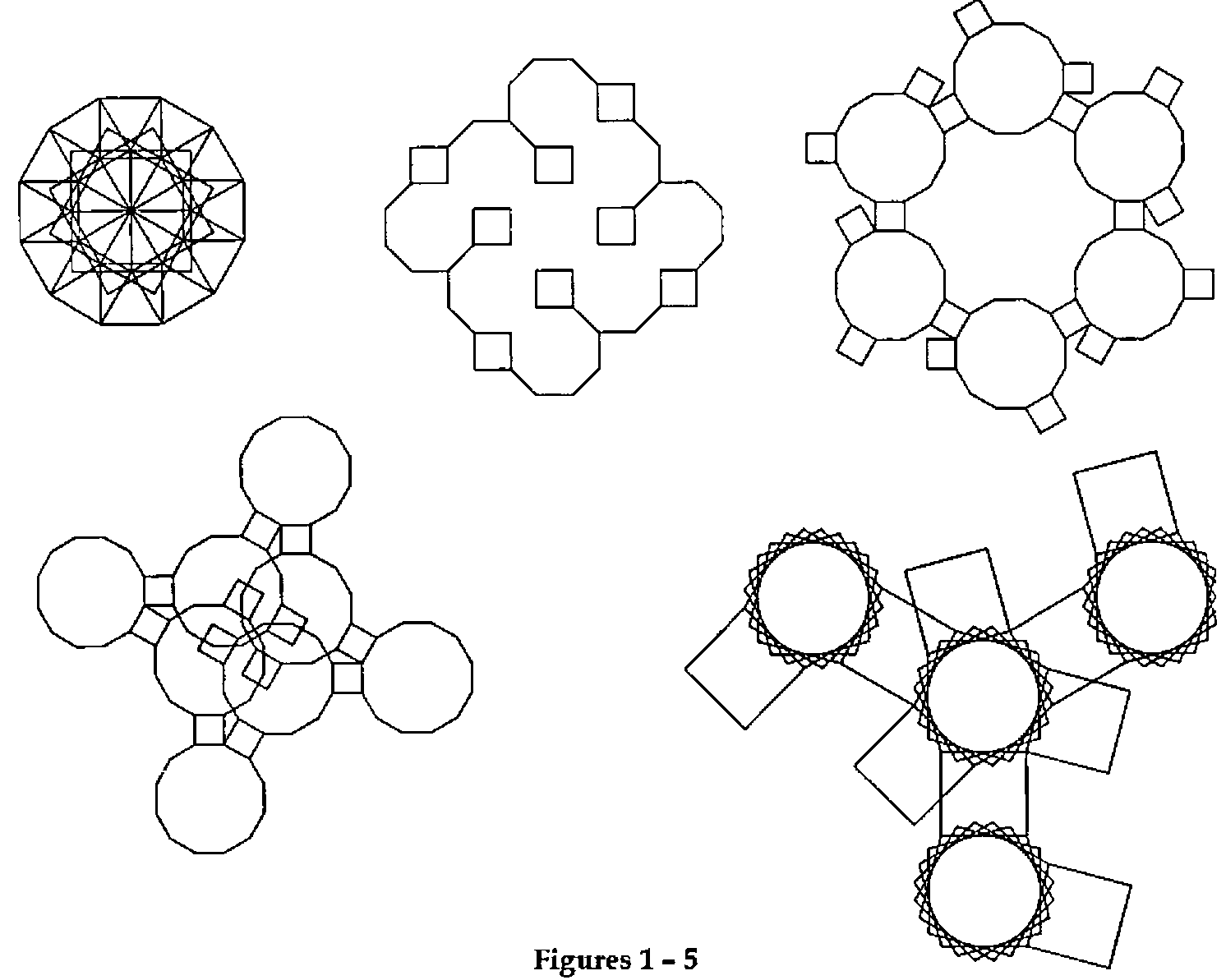
Five rosettes of polygons and squares

Figures 1 – 5

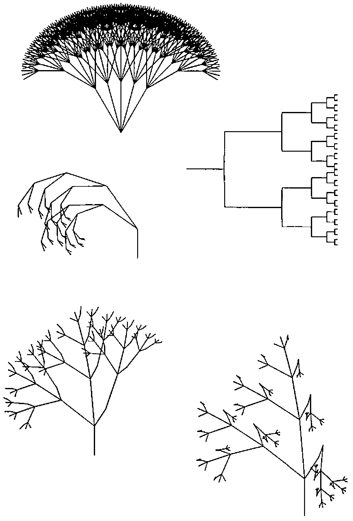
Five trees: a fan of branches, a binary tree, a curled tree and two irregular trees

Figures 6 – 10

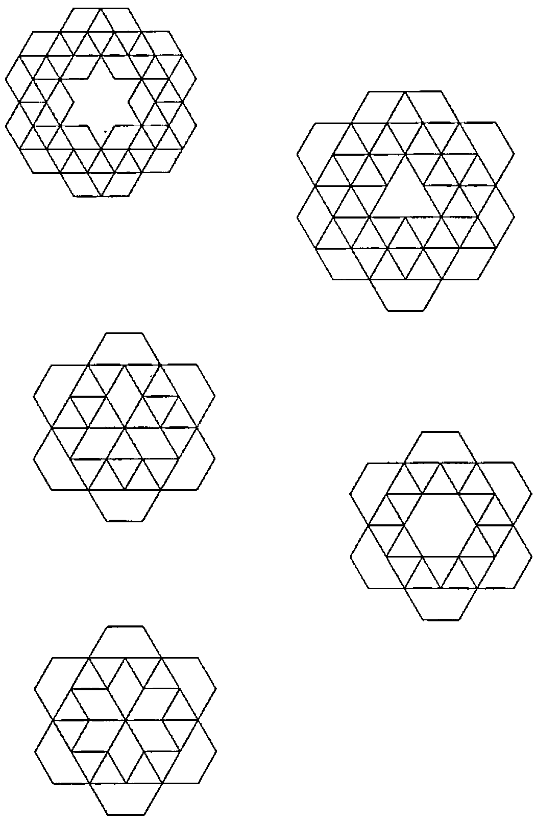
Five hexagonal patchworks of triangles and hexagons

Figures 11 – 15

References¶

[1] Harold Abalson & Andrea diSessa: Turtle Geometry, MIT Press, 1986

[2] Manuel Alfonseca: Representation of Fractal Curves by Means of L Systems, APL96, Lancaster (see www.demon.co.uk/apl385/apl96)