Swinging with APL: the Simple Pendulum

by Joseph De Kerf (Reprinted from APL-CAM Journal, Vol.18 No.1)

Transcribed from the printed issue; not yet reviewed. Read it in the PDF of the issue, page 128

Abstract¶

Calculation of time \(t\) as a function of the declination \(\theta\) of the simple pendulum with length \(l\) is reduced to the calculation of an incomplete elliptic integral of the first kind \(K(\phi;p)\). For the period \(T\) this is reduced to the calculation of a complete elliptic integral of the first kind \(K(p)\). Algorithms, based on the common mean concept, are illustrated with APL user-defined functions. Examples are given.

Introduction¶

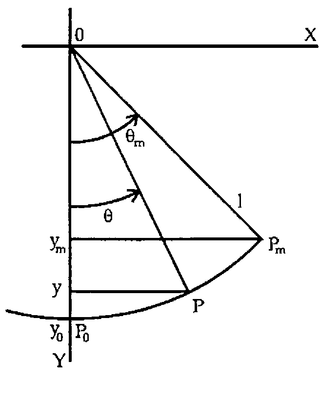
The simple pendulum: axes 0X and 0Y, the rod of length l from 0 to P at declination θ and to Pm at amplitude θm, the arc through P0, and heights y0, y and ym on the vertical axis

In a previous paper [1], we have shown that the rectification of a lot of so-called closed curves is reduced to the calculation of elliptic integrals. The elliptic integrals were evaluated with algorithms based on the common mean concept [2], as such algorithms are much more efficient in cpu time than those based on gaussian quadrature or serious expansion. Implementation was illustrated with APL user-defined functions, calling the user-defined functions described in [3] and [4]. In this paper, we follow the same line of thought for the solution of the simple or plane pendulum: the calculation of time \(t\) as a function of the declination \(\theta\) [5].

The Simple Pendulum¶

The simple or plane pendulum consists of a mass point \(m\) (\(P\)) at one end of a massless rigid rod with length \(l\), pivoted at the other end (0) and placed in a uniform gravitational field \(g\). Let \(P\) (declination \(\theta\)) be moving from the equilibrium position \(P_0\) (declination 0) towards its maximum displacement \(P_m\) (maximum declination or amplitude \(\theta_m\)).

Time versus Declination¶

\[\begin{alignat*}{2} &\text{Kinetic energy of the system is:}\qquad && \begin{alignedat}[t]{2} & \frac{1}{2}mv^2 &\qquad& \text{with} \\ & v = \frac{ds}{dt} && \text{and}\quad s = l\theta\left(v = l\frac{d\theta}{dt}\right) \end{alignedat} \\[1.5ex] &\text{Potential energy of the system is:} && \begin{alignedat}[t]{2} & mgl\,(1-\cos\theta) && \\ & \text{as } y_0 = l &\qquad& \text{and}\quad y = l\cos\theta \end{alignedat} \\[1.5ex] &\text{Conservation of energy gives:} && \frac{1}{2}mv^2 + mgl\,(1-\cos\theta) = mgl\,(1-\cos\theta_m) \\[1ex] &&& \frac{1}{2}mv^2 = mgl\,(\cos\theta-\cos\theta_m) \\[1ex] &&& v = \sqrt{2gl\,(\cos\theta-\cos\theta_m)} \\[1.5ex] &\text{Substituting } v \text{ by } l\frac{d\theta}{dt} \text{ we get:} && \frac{d\theta}{dt} = \sqrt{\frac{2g}{l}(\cos\theta-\cos\theta_m)} \\[1ex] &\hphantom{\text{Substituting } v \text{ by } l\frac{d\theta}{dt}}\text{or:} && dt = \sqrt{\frac{l}{2g}}\,\frac{d\theta}{\sqrt{\cos\theta-\cos\theta_m}} \end{alignat*}\]

Setting the time at the equilibrium point \(t_0 = 0\), time \(t\) for declination \(\theta\) becomes:

\[\begin{equation*} t = \sqrt{\frac{l}{2g}}\int_0^{\theta}\frac{d\theta}{\sqrt{\cos\theta-\cos\theta_m}} \end{equation*}\]

\[\begin{alignat*}{2} &\text{Substituting:}\qquad && \sin\frac{\theta}{2} = p\sin\phi \quad\text{with}\quad p = \sin(\theta_m/2) \\[1ex] &&& d\theta = \frac{2p\cos\phi}{\sqrt{1-p^2\sin^2\phi}}\,d\phi \\[1.5ex] &\text{we have:} && \sqrt{\cos\theta-\cos\theta_m} = \sqrt{2\bigl(\sin^2(\theta_m/2)-\sin^2(\theta/2)\bigr)} \\ &&& \hphantom{\sqrt{\cos\theta-\cos\theta_m}} = \sqrt{2}\,p\cos\phi \\[1.5ex] &\text{such that:} && t = \sqrt{\frac{l}{g}}\int_0^{\phi}\frac{d\phi}{\sqrt{1-p^2\sin^2\phi}} \quad=\quad \sqrt{\frac{l}{g}}\,K(\phi;p) \end{alignat*}\]

\(K(\phi;p)\) being the incomplete elliptic integral of the first kind with

\[\begin{equation*} \phi = \operatorname{arc\,sin}\left(\frac{\sin(\theta/2)}{p}\right) \quad\text{and}\quad p = \sin(\theta_m/2). \end{equation*}\]

APL Function¶

An APL user-defined function TIME for calculating time \(t\) as a function of the declination \(\theta\) may be:

      ∇TIME[⎕]∇
    ∇T←LA TIME D;F;P
[1]   F←((1↑LA)÷980.6294)*0.5
[2]   P←1○○(1↓LA)÷360
[3]   T←F×(¯1○(1○○D÷360)÷P) IEI1 P
    ∇

with: LA being the catenation of the length \(l\) (cm) and the maximum declination or amplitude \(\theta_m\) (degrees°)

D the declination \(\theta\) (degrees°)
P the parameter \(p = \sin(\theta_m/2)\)
F the factor \(\sqrt{l/g}\)
IEI1 the user-defined function described in [4]

and geodetic constant \(g\) being set to 980.6294cm/sec² (Hayford latitude 45°) [6].

\[\begin{alignat*}{2} \text{Example:}\qquad & l && = 100\,\text{cm} \\ & \theta_m && = 60^\circ \\ & \theta && = 10^\circ(10^\circ)60^\circ \end{alignat*}\]

      LA←100 60
      D←10×⍳6
      2 0 12 6 ⍕ D,⊃(6⍴⊂LA) TIME¨ D
10  0.056021
20  0.113851
30  0.175831
40  0.245926
50  0.333733
60  0.538320

Note:¶

The time to go from position \(P_0\) to maximum displacement \(P_m\) (\(\theta = \theta_m\) or \(\phi = \pi/2\)) is one-fourth of the period \(T\). Therefore, the period of the pendulum is:

\[\begin{align*} T &= 4\sqrt{\frac{l}{g}}\int_0^{\pi/2}\frac{d\phi}{\sqrt{1-p^2\sin^2\phi}} \\ &= 4\sqrt{\frac{l}{g}}\,K(p) \end{align*}\]

with \(p = \sin(\theta_m/2)\) and \(K(p)\) being the complete elliptic integral of the first kind.

The period \(T\) may be calculated with the function TIME, setting the right argument to the maximum declination or amplitude \(\theta_m\), and multiplying the result by 4. An APL user-defined function PERIOD for calculating the period directly from the complete elliptic integral of the first kind, more efficient in cpu time, may be:

      ∇PERIOD[⎕]∇
    ∇T←L PERIOD A;F;P
[1]   F←(L÷980.6294)*0.5
[2]   P←1○○A÷360
[3]   T←4×F×CEI1 P
    ∇

with: L being the length \(l\) (cm)

A the maximum declination of amplitude \(\theta_m\) (degrees °)
CEI1 the user-defined function described in [3]

and the geodetic constant \(g\) being set to 980.6294cm/sec² (Hayford latitude 45°) [6]. The period \(T\) is returned in seconds.

\[\begin{alignat*}{2} \text{Example:}\qquad & l && = 100\,\text{cm} \\ & \theta_m && = 60^\circ \end{alignat*}\]

      8 6 ⍕ 4×100 60 TIME 60
2.153281
      8 6 ⍕ 100 PERIOD 60
2.153281

References¶

J. De Kerf: Rectification with APL; APL-CAM Journal, Vol. 17, No. 4, 16th December 1995 pp. 560 - 582.
J. De Kerf: The Common Mean and APL; APL-CAM Journal, Vol. 16, No. 3, 16th July 1994, pp. 370 - 372.
See also: Vector, Vol. 11, No. 3, January 1995, pp. 21 - 23.
J. De Kerf: The Complete Elliptic Integrals and APL; APL-CAM Journal, Vol. 16, No. 4, 16th October 1994, pp. 631 - 635.
See also: Vector, Vol. 12, No. 1, July 1995, pp. 102 - 106.
J. De Kerf: The Incomplete Elliptic Integrals and APL - An Extension; APL-CAM Journal, Vol. 17, No. 3, 16th September 1995, pp. 455 - 460.
See also: Vector, Vol. 12, No. 2, October 1995, pp. 95 - 100.
H.C. Corben and P. Stehle: Classical Mechanics; John Wiley & Sons, New York, 1950.
M.Abramowitz and L.A. Stegun (eds.): Handbook of Mathematical Functions; Applied Mathematics Series No. 55; National Bureau of Standards, Washington D.C., 1964 (and subsequent revisions).

Appendix¶

For convenience of the reader, the APL user-defined functions CEI1 [3] and IEI1 [4], referred to in this paper, are reproduced here:

      ∇CEI1[⎕]∇
    ∇R←CEI1 P
[1]   R←1,(1-P*2)*0.5
[2]   LAB:→(≠/R←(0.5×+/R),(×/R)*0.5)/LAB
[3]   R←(○1)÷+/R
    ∇

      ∇IEI1[⎕]∇
    ∇R←F IEI1 P;I;A;B
[1]   →((1≠|P)∨(○÷2)≤|F)/LAB1
[2]   →0,R←⍟3○0.5×F+○0.5
[3]   LAB1:R←(2+I←¯1),÷÷(1-P*2)*0.5
[4]   LAB2:A←(-/R)×1○F×2*1+I←I+1
[5]   B←2×+/R×(2 1○F×2*I)*2
[6]   F←F-(¯3○A÷B)÷2*I+1
[7]   →(≠/R←(0.5×+/R),(×/R)*0.5)/LAB2
[8]   R←F÷0.5×+/R
    ∇